Utilizing LIGER for the integration of spatial transcriptomic data
Joshua Sodicoff
7/17/2020
Source:vignettes/birs_revised.Rmd
birs_revised.RmdUpdates
This vignette will differ somewhat from my original presentation, namely in that it does not require access to any datasets outside of those provided for the hackathon. Likewise, instead of comparing an analysis across spatial modalities, it will demonstrate the method for generating the results required for that on the conference data. I hope this vignette helps you learn how to use Liger for this task and interpret UMAP plots and clustering metrics to determine the accuracy of your integration
Overview
In this analysis, the additional structure found by combining spatial and single cell transcriptomic datasets with an integrative nonnegative matrix factorization-based method, Liger, is demonstrated. From the separate and integrative analyses, plots of identified and known clusters are generated, metrics of integration performance are compared in context, and it is shown that there is some loss of information as a result of the integration.
#Viewing the data
First, let’s preview the data to ensure that gene features comprise the rows, samples comprise the columns, and known cluster assignments are factor vectors.
tasic[1:10,1:10]
##          tasic_1 tasic_2 tasic_3 tasic_4 tasic_5 tasic_6 tasic_7 tasic_8
## abca15        11      42      17      42      35      35      35      42
## abca9         22      46      22      46      39      39      39      46
## acta2         15      47      15      42      34      42      34      47
## adcy4         12      45      12      45      38      38      38      45
## aldh3b2       27      49      27      49      42      42      49      49
## amigo2        23      43     101      43      72      43      43      49
## ankle1        29      46      72      37      61      35      41      24
## ano7          11      42      16      42      34      34      34      42
## anxa9         15      48      15      42      33      42      33      42
## arhgef26      59      43      75      43      36      43      85      49
##          tasic_9 tasic_10
## abca15        48       35
## abca9         46       39
## acta2         47       42
## adcy4         45       38
## aldh3b2       49       42
## amigo2        49       43
## ankle1        49       48
## ano7          48       34
## anxa9         48       42
## arhgef26 49 54tasic_clust[1:10]
##   tasic_1   tasic_2   tasic_3   tasic_4   tasic_5   tasic_6   tasic_7   tasic_8
## Astrocyte Astrocyte Astrocyte Astrocyte Astrocyte Astrocyte Astrocyte Astrocyte
##   tasic_9  tasic_10
## Astrocyte Astrocyte
## 8 Levels: Astrocyte Endothelial Cell ... Oligodendrocyte.3seqfish[1:10,1:10]
##          seqfish_1 seqfish_2 seqfish_3 seqfish_4 seqfish_5 seqfish_6 seqfish_7
## abca15          68        49        50        39        31        59        44
## abca9           41        42        38        36        47        18        37
## acta2           25        23        16        21        29        36        21
## adcy4           39        54        37        18        37        26        36
## aldh3b2        101        47        41        52       101        50       101
## amigo2          93        64        93        93        93        93        63
## ankle1          41        42        76        40        46        38        63
## ano7            44        68        50        48        50        46        41
## anxa9           53        40        43        39        31        39        36
## arhgef26        38        40        42        45        46        44        37
##          seqfish_8 seqfish_9 seqfish_10
## abca15          66        50         46
## abca9           48        31         41
## acta2           32        25         11
## adcy4           32        33         40
## aldh3b2         56        40         42
## amigo2          56        93         62
## ankle1          27         9         41
## ano7            37        31         46
## anxa9           36        44         82
## arhgef26 45 28 42seq_clust[1:10]
##            seqfish_1            seqfish_2            seqfish_3
## Glutamatergic Neuron Glutamatergic Neuron Glutamatergic Neuron
##            seqfish_4            seqfish_5            seqfish_6
## Glutamatergic Neuron Glutamatergic Neuron Glutamatergic Neuron
##            seqfish_7            seqfish_8            seqfish_9
## Glutamatergic Neuron Glutamatergic Neuron Glutamatergic Neuron
##           seqfish_10
## Glutamatergic Neuron
## 8 Levels: Astrocyte Endothelial Cell ... Oligodendrocyte.3
Separate integrations
To establish a baseline as the level of structure and clustering accuracy that can be found for each dataset with LIGER, we run individual analyses.
The analysis includes 1. Normalization, to standardize the counts per sample 2. Variable gene selection 3. Scaling, but not centering as not to violate the nonnegativity constraint 4. Integrative non-negative matrix factorization, or essentially just NMF in the case shown here in which one dataset is provided 5. Quantile normalization, primarily used for aligning multiple datasets. 6. Cluster identification with the Louvain algorithm 7. UMAP, for visualization
First, we run the analysis on the scRNA-seq data
tasic_obj = createLiger(list(sc_rnaseq = tasic))
tasic_obj %<>% liger::normalize() %>%
    liger::selectGenes() %>%
    liger::scaleNotCenter() %>%
    liger::optimizeALS(k = 20) %>%
    liger::quantile_norm() %>%
    liger::louvainCluster() %>%
    liger::runUMAP()
Then, we run it on the seqFISH data
seq_obj = createLiger(list(spatial = seqfish))
seq_obj %<>% liger::normalize() %>%
    liger::selectGenes() %>%
    liger::scaleNotCenter() %>%
    liger::optimizeALS(k = 20) %>%
    liger::quantile_norm() %>%
    liger::louvainCluster() %>%
    liger::runUMAP()
We then plot the evaluated data by generated and known cluster for the scRNA-seq
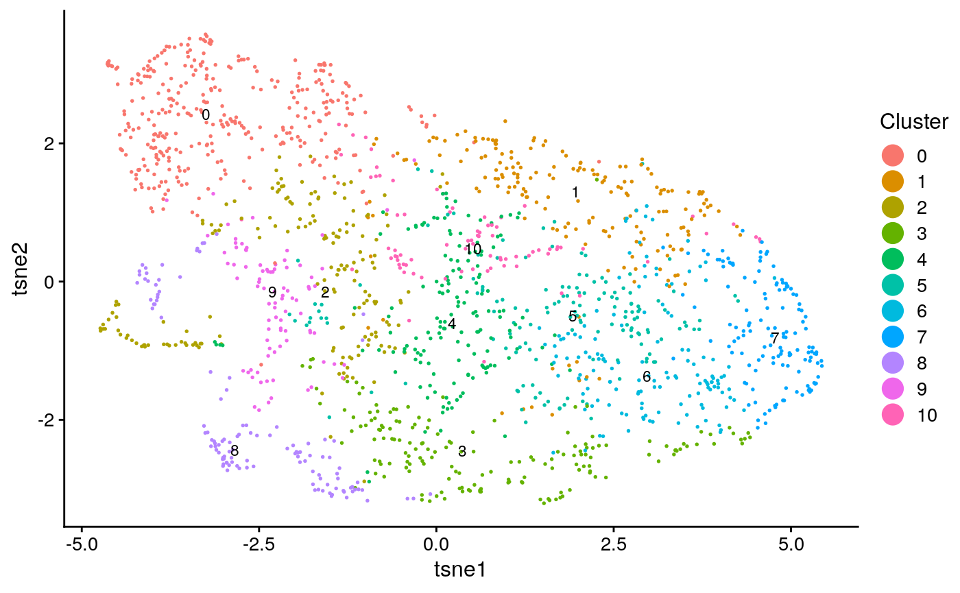
names(tasic_obj@clusters) = colnames(tasic)
tasic_plots = plotByDatasetAndCluster(tasic_obj, return.plots = T)
tasic_plot_known_clust = plotByDatasetAndCluster(tasic_obj, clusters = tasic_clust, return.plots = T)
tasic_plots[[2]]
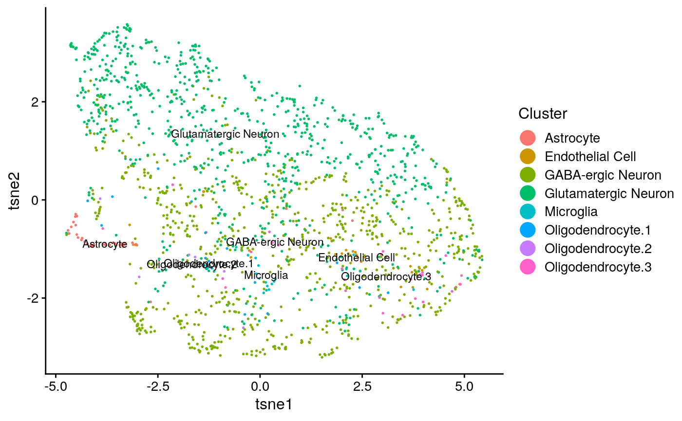
tasic_plot_known_clust[[2]]
 and then the spatial data
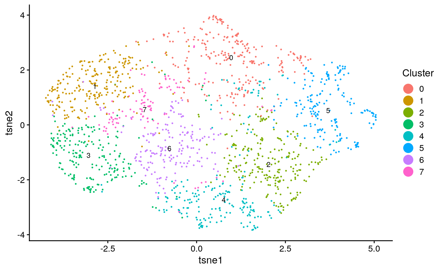
names(seq_obj@clusters) = colnames(seqfish)
seq_plots = plotByDatasetAndCluster(seq_obj, return.plots = T)
seq_plot_known_clust = plotByDatasetAndCluster(seq_obj, clusters = seq_clust, return.plots = T)
seq_plots[[2]]
seq_plot_known_clust[[2]]
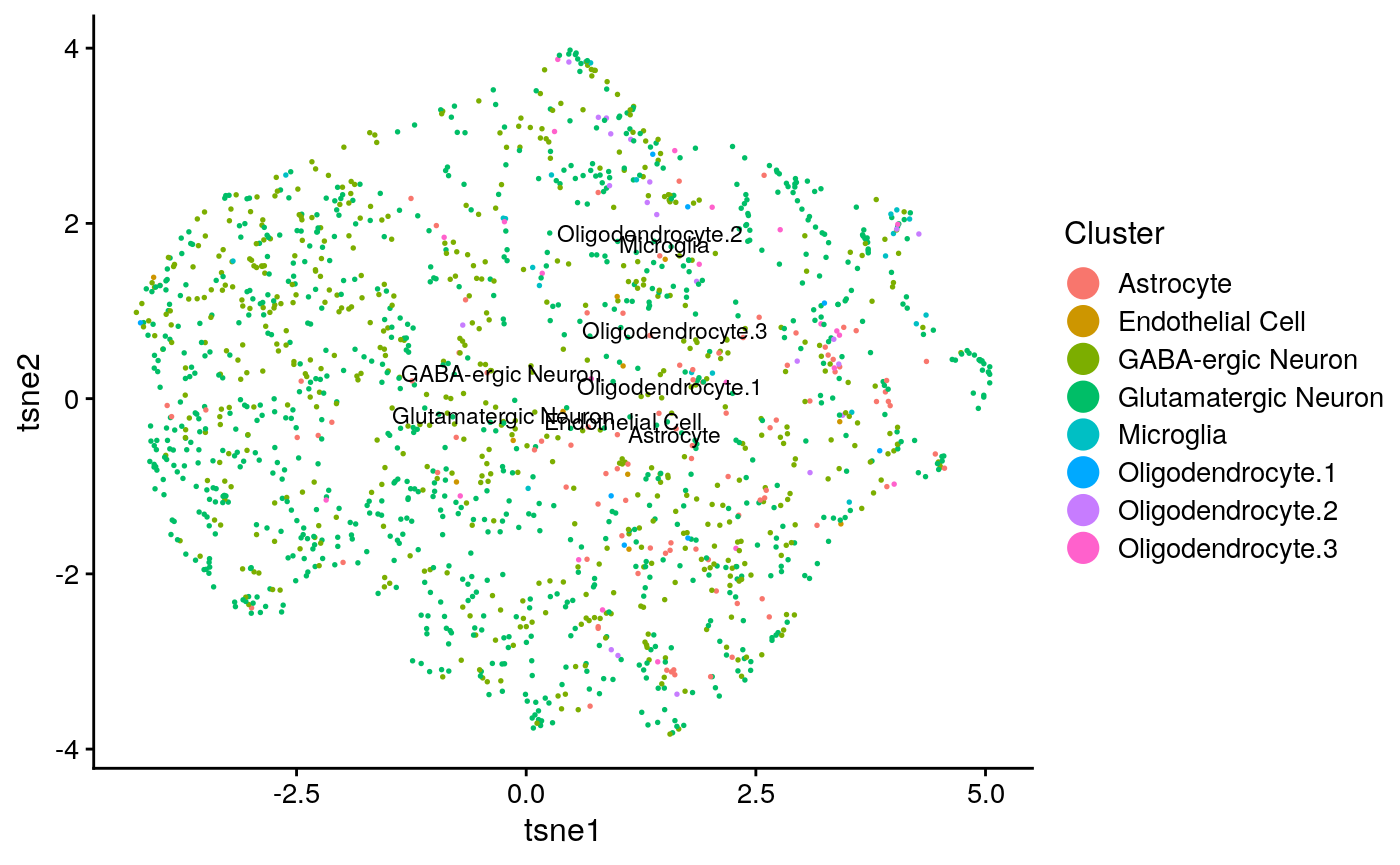 We can make a few qualitative obeservations: * Neither analysis seems to have a lot of structure, resulting in the UMAP plots coming out rather “blobby”. * The known clusters in the scRNA-seq seem to map slightly better to the generated clusters than the spatial data.
We calculate metrics of clustering accuracy to compare. ARI is the adjusted Rand index, a metric based on the number of cell-cell pairs known to reside in the same and different clusters and adjusted to account for random chance. Purity is found by dividing the total number of correctly identified cells in a cluster over the total number of cells in that cluster.
## [1] "tasic ARI: 0.124928479183329"## [1] "tasic purity: 0.737086477074869"## [1] "seqfish ARI: 0.00922479431962868"## [1] "seqfish purity: 0.546023794614903"This confirms that the single cell data had somewhat better clustering accuracy.
Now, let’s try to integrate the datasets, using almost the same workflow as before but with both datasets provided for object creation.
int_obj = createLiger(list(sc_rnaseq = tasic, spatial = seqfish))
int_obj %<>% liger::normalize() %>%
    liger::selectGenes() %>%
    liger::scaleNotCenter() %>%
    liger::optimizeALS(k = 20) %>%
    liger::quantile_norm() %>%
    liger::louvainCluster() %>%
    liger::runUMAP()
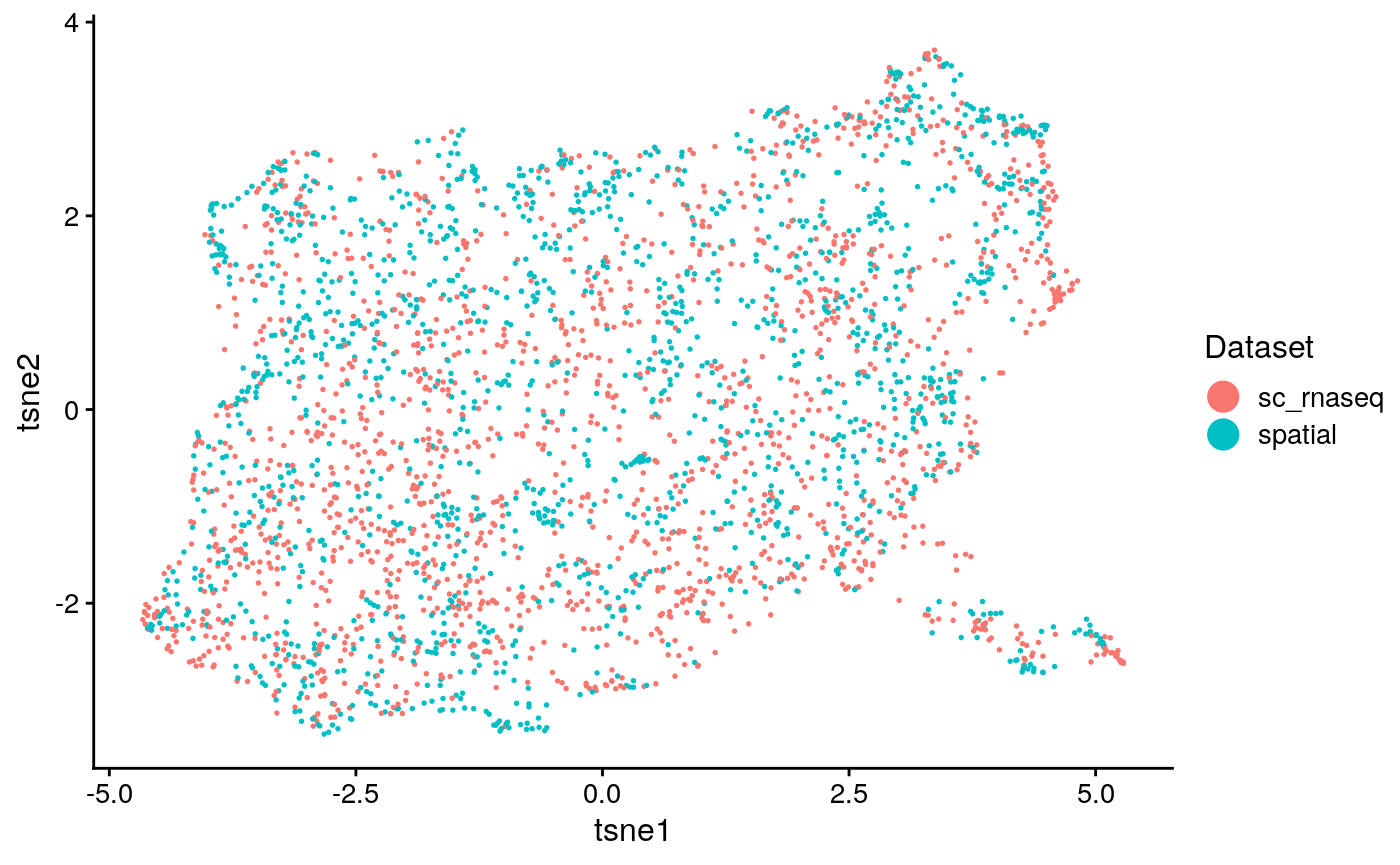
Again, we plot the output, including one showing dataset of origin
names(int_obj@clusters) = c(colnames(tasic), colnames(seqfish))
int_clust = as.factor(c(as.character(tasic_clust), as.character(seq_clust))); names(int_clust) = c(names(tasic_clust), names(seq_clust))
int_plots = plotByDatasetAndCluster(int_obj, return.plots = T)
int_plot_known_clust = plotByDatasetAndCluster(int_obj, clusters = int_clust, return.plots = T)
int_plots[[1]]
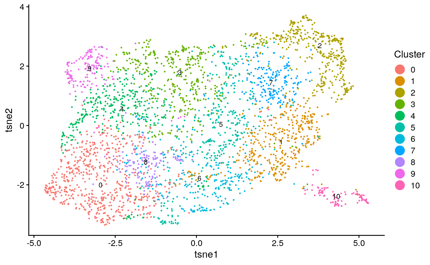
int_plots[[2]]
int_plot_known_clust[[2]]
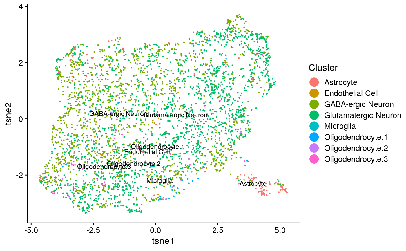
We calculate clustering accuracy, as well as agreement and alignment
## [1] "overall ARI: 0.03990832682262"## [1] "overall purity: 0.621084337349398"## [1] "Reducing dimensionality using NMF"
##
## Converged in 0.01860118 seconds, 167 iterations. Objective: 5408.016
##
## Converged in 0.01765323 seconds, 188 iterations. Objective: 8577.805
## [1] "agreement: 0.089592886480605"## [1] "alignment: 0.804064439004953"This seems to demonstrate that the clustering accuracy of the integration (a surrogate for how well the method divided the cell types) falls somehwere between solely using the spatial data and scRNA-seq. Additionally, the agreement metric is relatively low (on its scale of 0 to 1). This implies that the integration was not very informative and relied heavily on distortion of the data for alignment.